.ipynb .pdf

repository open issue suggest edit

Binder

Contents

Quick start

This notebook is for a quick start to plot basic result from the G50 fabric analyser.

import xarrayaita.loadData_aita as lda #here are some function to build xarrayaita structure
import xarrayaita.aita as xa
import xarrayuvecs.uvecs as xu
import xarrayuvecs.lut2d as lut2d

import matplotlib.pyplot as plt
import matplotlib.cm as cm
import numpy as np

Load your data

# path to data and microstructure
path_data='orientation_test.dat'
path_micro='micro_test.bmp'

data=lda.aita5col(path_data,path_micro)

data

<xarray.Dataset>
Dimensions:      (uvecs: 2, x: 1000, y: 2500)
Coordinates:
  * x            (x) float64 0.0 0.02 0.04 0.06 0.08 ... 19.92 19.94 19.96 19.98
  * y            (y) float64 49.98 49.96 49.94 49.92 49.9 ... 0.06 0.04 0.02 0.0
Dimensions without coordinates: uvecs
Data variables:
    orientation  (y, x, uvecs) float64 2.395 0.6451 5.377 ... 0.6098 0.6473
    quality      (y, x) int64 0 90 92 93 92 92 94 94 ... 96 96 96 96 96 97 97 96
    micro        (y, x) float64 0.0 0.0 0.0 0.0 0.0 0.0 ... 0.0 0.0 0.0 0.0 0.0
    grainId      (y, x) int64 1 1 1 1 1 1 1 1 1 1 1 1 ... 1 1 1 1 1 1 1 1 1 1 1
Attributes:
    date:       Thursday, 19 Nov 2015, 11:24 am
    unit:       millimeters
    step_size:  0.02
    path_dat:   orientation_test.dat

With G50 fabric analyser we usually filter the value with a quality below \(75\).

data.aita.filter(75)

Plot colormap

Plotting a colormap using a color wheel is done using xarrayuvecs

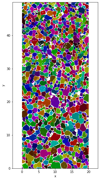
Full colorwheel

data['FullColormap']=data.orientation.uvecs.calc_colormap()

Therfore the FullColormap variable is store in the xarray.Dataset

data

<xarray.Dataset>
Dimensions:       (img: 3, uvecs: 2, x: 1000, y: 2500)
Coordinates:
  * x             (x) float64 0.0 0.02 0.04 0.06 ... 19.92 19.94 19.96 19.98
  * y             (y) float64 49.98 49.96 49.94 49.92 ... 0.06 0.04 0.02 0.0
Dimensions without coordinates: img, uvecs
Data variables:
    orientation   (y, x, uvecs) float64 nan nan 5.377 ... 0.6395 0.6098 0.6473
    quality       (y, x) int64 0 90 92 93 92 92 94 94 ... 96 96 96 96 97 97 96
    micro         (y, x) float64 0.0 0.0 0.0 0.0 0.0 0.0 ... 0.0 0.0 0.0 0.0 0.0
    grainId       (y, x) int64 1 1 1 1 1 1 1 1 1 1 1 1 ... 1 1 1 1 1 1 1 1 1 1 1
    FullColormap  (y, x, img) float64 255.0 255.0 255.0 0.0 ... 0.0 0.425 0.1756
Attributes:
    date:       Thursday, 19 Nov 2015, 11:24 am
    unit:       millimeters
    step_size:  0.02
    path_dat:   orientation_test.dat

The plot can be done using :

plt.figure(figsize=(5,10))
data.FullColormap.plot.imshow()
plt.axis('equal')

Clipping input data to the valid range for imshow with RGB data ([0..1] for floats or [0..255] for integers).

(-0.01, 19.990000000000002, -0.010000000000001563, 49.99000000000001)

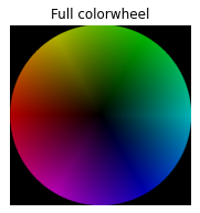
The associated colorwheel can be plot using :

lut_f=lut2d.lut()

plt.figure(figsize=(3,3))
plt.imshow(lut_f)
plt.axis('equal')
plt.axis('off')
plt.title('Full colorwheel')

Text(0.5, 1.0, 'Full colorwheel')

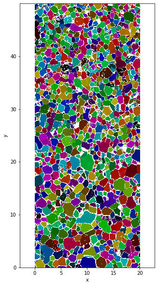
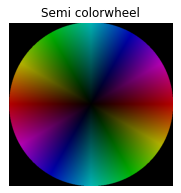
Semi colorwheel

The same figure can be done using a “semi” colorwheel.

Warning

\((x,y,z)\) and \((-x,-y,z)\) share the same colorcoding.

data['SemiColormap']=data.orientation.uvecs.calc_colormap(semi=True)

plt.figure(figsize=(5,10))
data.SemiColormap.plot.imshow()
plt.axis('equal')

Clipping input data to the valid range for imshow with RGB data ([0..1] for floats or [0..255] for integers).

(-0.01, 19.990000000000002, -0.010000000000001563, 49.99000000000001)

lut_s=lut2d.lut(semi=True)
plt.figure(figsize=(3,3))
plt.imshow(lut_s)
plt.axis('equal')
plt.axis('off')
plt.title('Semi colorwheel')

Text(0.5, 1.0, 'Semi colorwheel')

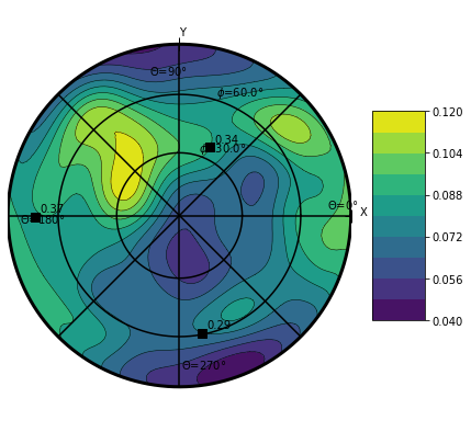
Plot ODF

ODF stand for Orientation Density Function. It is a probability density function for orientation. Therefore it’s integral over the sphere is equal to 1.

Warning

The plotODF function is very quite sensible to the bw input parameter that is the bandwidth of kernel for the kde estimation. See documentation here (Need to document this in xarrayuvecs)

The ODF

plt.figure(figsize=(7,7))
data.orientation.uvecs.plotODF(bw=0.2,cmap=cm.viridis)

The 2nd order orientation tensor

The second order orientation tensor of a set of \(x_i\) vector is defnied by :

\(OT2nd=\frac{1}{N}\sum_{i=1}^{N}x_i \otimes x_i\)

There for you can extract the eigen value and eigen vector of it. It is what xu.uvec.OT2nd does.

e_val,e_vec=data.orientation.uvecs.OT2nd()
print('The 1st eigen value is :',e_val[0],'. Associated with the vector :',e_vec[:,0] )
print('The 2nd eigen value is :',e_val[1],'. Associated with the vector :',e_vec[:,1] )
print('The 3rd eigen value is :',e_val[2],'. Associated with the vector :',e_vec[:,2] )

The 1st eigen value is : 0.36842623 . Associated with the vector : [ 0.95692456  0.00752591 -0.29023907]
The 2nd eigen value is : 0.3406706 . Associated with the vector : [0.24083522 0.5377383  0.8079826 ]
The 3rd eigen value is : 0.2909032 . Associated with the vector : [-0.16215347  0.8430782  -0.5127625 ]

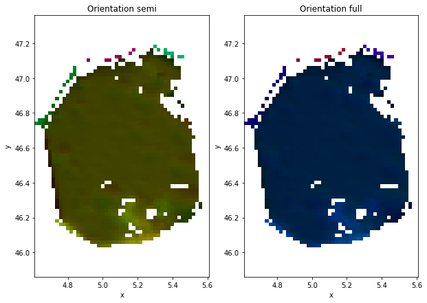
Work on subset

Only on grain

gId=100

ds=data.where(data.grainId==gId,drop=True)

plt.figure(figsize=(10,7))
plt.subplot(1,2,1)
ds.SemiColormap.plot.imshow()
plt.axis('equal')
plt.title('Orientation semi')
plt.subplot(1,2,2)
ds.FullColormap.plot.imshow()
plt.axis('equal')
plt.title('Orientation full')

Clipping input data to the valid range for imshow with RGB data ([0..1] for floats or [0..255] for integers).

Clipping input data to the valid range for imshow with RGB data ([0..1] for floats or [0..255] for integers).

Text(0.5, 1.0, 'Orientation full')

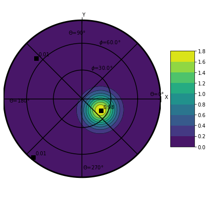
plt.figure(figsize=(7,7))
ds.orientation.uvecs.plotODF(nbr=100)

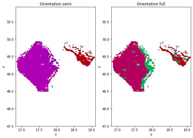
More grains

ds2=data.where((data.grainId==4)+(data.grainId==5),drop=True)

plt.figure(figsize=(10,7))
plt.subplot(1,2,1)
ds2.SemiColormap.plot.imshow()
plt.axis('equal')

plt.title('Orientation semi')
plt.subplot(1,2,2)
ds2.FullColormap.plot.imshow()
plt.axis('equal')

plt.title('Orientation full')

Clipping input data to the valid range for imshow with RGB data ([0..1] for floats or [0..255] for integers).

Clipping input data to the valid range for imshow with RGB data ([0..1] for floats or [0..255] for integers).

Text(0.5, 1.0, 'Orientation full')

Welcome to AITA book Crop data