The `xarray.DataArray` stucture for uvecs¶

xarrayuvecs propose a accessor for xarray.DataArray to work on “Unit VECctor that are Symmetrical” (UVECS).

In this case symetrical mean that a vector x has the same meaning than -x. Therefore is can be usefull to describe non directional orientation such as crystallographic orientation dor instance.

In this notebook we will show what can be done using xarrayuvec accessor.

import xarrayaita.loadData_aita as lda #here are some function to build xarrayaita structure
import xarrayaita.aita as xa
import xarrayuvecs.uvecs as xu
import xarrayuvecs.lut2d as lut2d

import numpy as np
import matplotlib.pyplot as plt
import matplotlib.cm as cm
import xarray as xr

Load data

# path to data and microstructure
path_data='orientation_test.dat'
path_micro='micro_test.bmp'

data=lda.aita5col(path_data,path_micro)

What is an `xarrayuvecs` `DataArray` ?¶

data.orientation.head(2)

<xarray.DataArray 'orientation' (y: 2, x: 2, uvecs: 2)>
array([[[2.39476627, 0.64507369],
        [5.37718489, 1.04999008]],

       [[5.35955707, 1.15837502],
        [5.35885894, 1.12975162]]])
Coordinates:
  * x        (x) float64 0.0 0.02
  * y        (y) float64 49.98 49.96
Dimensions without coordinates: uvecs

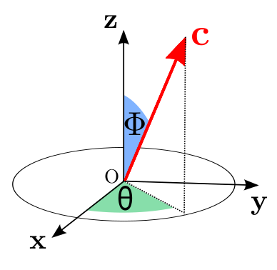
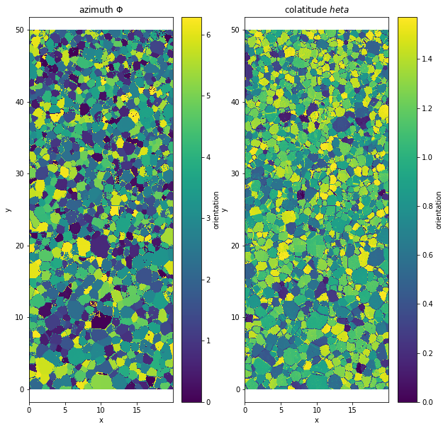
xarrayuvecs accessor should be used on xarray.DataArray da that have a dimension of \(m\times n \times 2\). The da[:,:,0] correspond to the azimuth \(\Phi\) coordinate of the unit vector and da[:,:,1] to the colatitude \(\theta\).

Definition of the Azimuth and Colatitude.}

plt.figure(figsize=(10,10))
plt.subplot(1,2,1)
data.orientation[:,:,0].plot()
plt.axis('equal')
plt.title('azimuth $\Phi$')
plt.subplot(1,2,2)
data.orientation[:,:,1].plot()
plt.axis('equal')
plt.title('colatitude $\theta$')

Text(0.5, 1.0, 'colatitude $\theta$')

../_images/The_dataArray_structure_10_1.png

Export different coordinate system¶

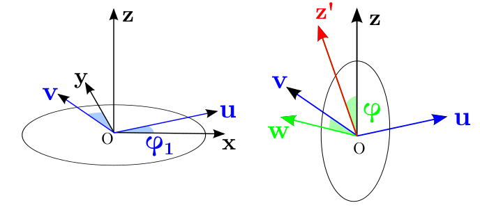
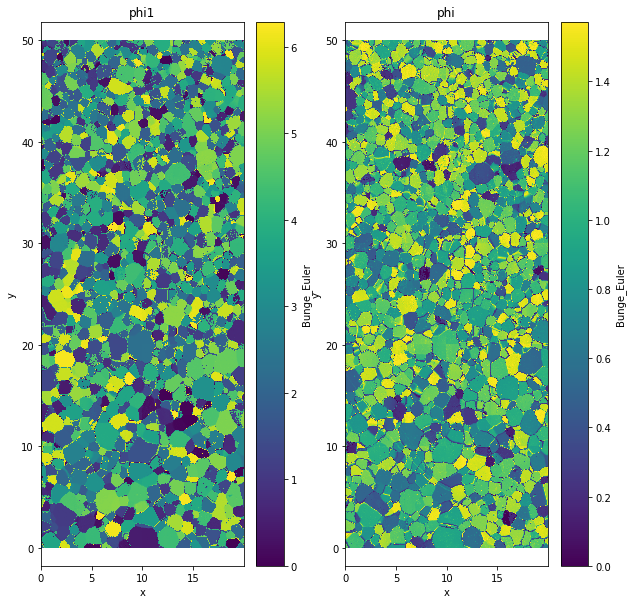
Bunge Euler convention¶

The Bunge Euler convention is widely use in crystallographic community.

\(\phi_1\) is the rotation around \(Oz\)
\(\phi\) is the rotation around \(Ou\)

Definition of the Bunge Euler angle.

data['Bunge_Euler']=data.orientation.uvecs.bunge_euler()

plt.figure(figsize=(10,10))
plt.subplot(1,2,1)
data.Bunge_Euler[:,:,0].plot()
plt.axis('equal')
plt.title('phi1')
plt.subplot(1,2,2)
data.Bunge_Euler[:,:,1].plot()
plt.axis('equal')
plt.title('phi')

Text(0.5, 1.0, 'phi')

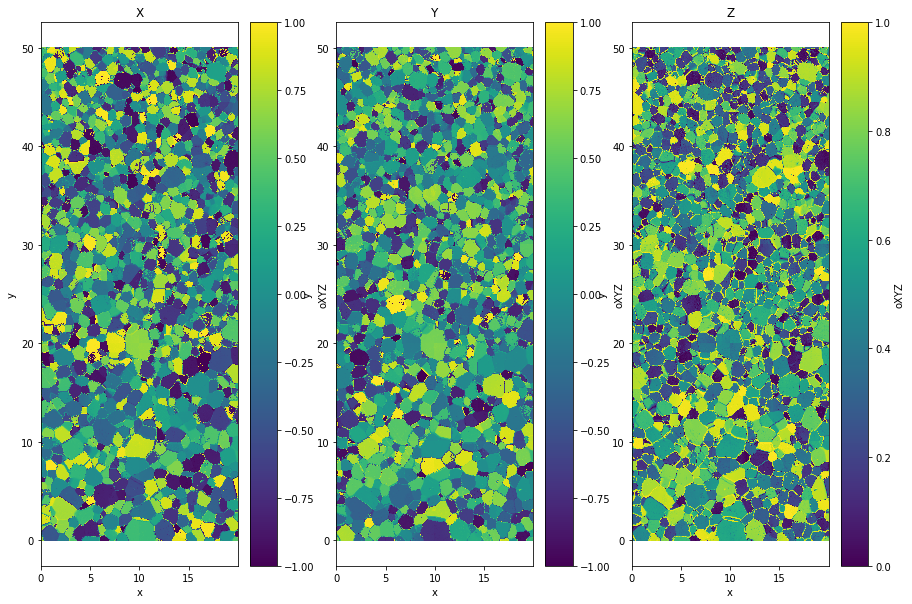
../_images/The_dataArray_structure_13_1.png

Cartesien coordinate¶

You can also extract the vector in cartesien coordinate.

data['oXYZ']=data.orientation.uvecs.xyz()

plt.figure(figsize=(15,10))
plt.subplot(1,3,1)
data.oXYZ[:,:,0].plot(cmap=cm.viridis)
plt.axis('equal')
plt.title('X')
plt.subplot(1,3,2)
data.oXYZ[:,:,1].plot(cmap=cm.viridis)
plt.axis('equal')
plt.title('Y')
plt.subplot(1,3,3)
data.oXYZ[:,:,2].plot(cmap=cm.viridis)
plt.axis('equal')
plt.title('Z')

Text(0.5, 1.0, 'Z')

../_images/The_dataArray_structure_16_1.png

Colormap¶

Colormap plotting the orientation can be done using colorwheel.

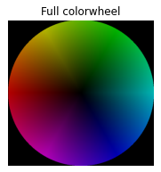
Full colorwheel¶

The colorcode used to display one orientation is choosen using a given colorwheel (show below). Using the “Full Colorwheel” will display a unique color for all the same orientation.

a black pixel display an orientation along the z-axis \((0,0,1)\)
a red pixel display an orientation along the minus x-axis \((-1,0,0)\)
a blue pixel display an orientation along the \(\left(\frac{\sqrt(2)}{2},\frac{-\sqrt(2)}{2},0\right)\)

This representation is quite usefull but is not exempt of default. For instance The color codding is discontinous. That mean that vectors \(\left(1,0,+\delta_z\right)\) and \(\left(1,0,-\delta_z\right)\) show very defferent color (pale blue and red) even if the angle between both decrease to 0 as \(\delta_z\) decrease to 0.

lut_f=lut2d.lut()
plt.figure(figsize=(3,3))
plt.imshow(lut_f)
plt.axis('equal')
plt.axis('off')
plt.title('Full colorwheel')

Text(0.5, 1.0, 'Full colorwheel')

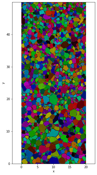
../_images/The_dataArray_structure_18_1.png

The colormap associated with this colorwheel can be compute using xarrayuvecs

data['FullColormap']=data.orientation.uvecs.calc_colormap()

plt.figure(figsize=(5,10))
data.FullColormap.plot.imshow()
plt.axis('equal')

(-0.01, 19.990000000000002, -0.010000000000001563, 49.99000000000001)

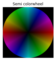
../_images/The_dataArray_structure_21_1.png

Semi colorwheel¶

The semi colorwheel is an over represntation of the orientation. It has the advantage to not have any discountinuities but one color does not correspond to a unique orientation.

Warning

\((x,y,z)\) and \((-x,-y,z)\) share the same colorcoding.

lut_s=lut2d.lut(semi=True)
plt.figure(figsize=(3,3))
plt.imshow(lut_s)
plt.axis('equal')
plt.axis('off')
plt.title('Semi colorwheel')

Text(0.5, 1.0, 'Semi colorwheel')

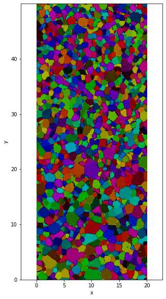
../_images/The_dataArray_structure_23_1.png

data['SemiColormap']=data.orientation.uvecs.calc_colormap(semi=True)

plt.figure(figsize=(5,10))
data.SemiColormap.plot.imshow()
plt.axis('equal')

(-0.01, 19.990000000000002, -0.010000000000001563, 49.99000000000001)

../_images/The_dataArray_structure_25_1.png

The ODF¶

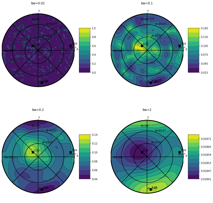
The Orientation Density Function (ODF) is a probability density function for orientation. Therefore it’s integral over the sphere is equal to 1.

It is evaluated using a Kernel Density Estimation (KDE) with a gaussian kernel.

Warning

Therefore the representation is quite sensitive to the ‘bandwidth’ bw paramerter of the gaussian kernel and should be choosen carefully.

plt.figure(figsize=(14,14))
plt.subplot(221)
data.orientation.uvecs.plotODF(bw=0.02,cmap=cm.viridis)
plt.title('bw=0.02')
plt.subplot(222)
data.orientation.uvecs.plotODF(bw=0.1,cmap=cm.viridis)
plt.title('bw=0.1')
plt.subplot(223)
data.orientation.uvecs.plotODF(bw=0.2,cmap=cm.viridis)
plt.title('bw=0.2')
plt.subplot(224)
data.orientation.uvecs.plotODF(bw=2.,cmap=cm.viridis)
plt.title('bw=2')

Text(0.5, 1.0, 'bw=2')

../_images/The_dataArray_structure_27_1.png

AITA data analysis

The xarray.DataArray stucture for uvecs¶

What is an xarrayuvecs DataArray ?¶